个体与集成
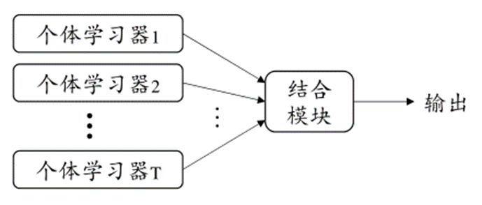
集成学习(ensemble learning)通过构建并结合多个学习器来提升性能
假设一个二分类问题,集成通过简单投票法结合T个分类器,每个基分类器错误率相互独立,则有Hoeffding不等式可得集成错误率为
\[P(H(x)\ne f(x))=\sum\limits_{i=1}^T \begin{pmatrix}T\\ k\end{pmatrix} (1-\epsilon)^k\epsilon^{T-k}\le exp(-\frac{1}{2}T(1-2\epsilon)^2)\]实际任务中,个体学习器是为了解决同一个问题训练出来的,不可能相互独立。个体学习器的“准确性”和“多样性”存在冲突,如何产生“好而不同”的个体学习器是集成学习的核心
集成学习大致分为两个大类
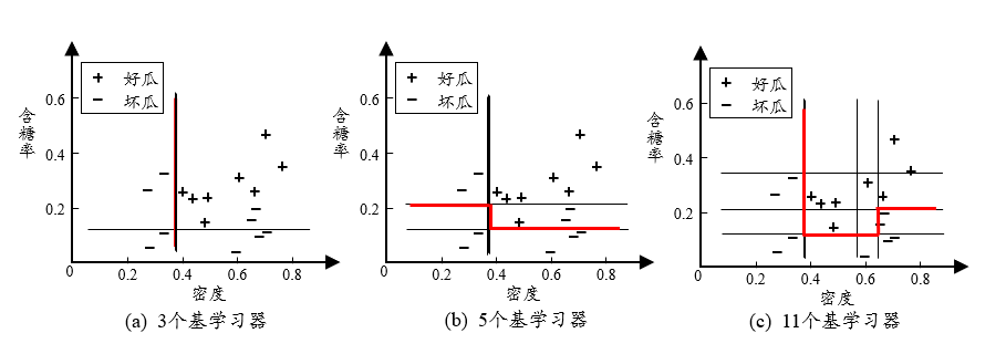
- Boosting
- Bagging
Boosting
- 个体学习器存在强依赖关系
- 串行生成
- 每次调整训练数据的样本分布
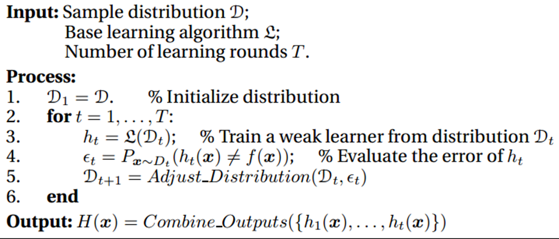
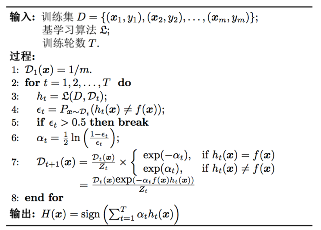
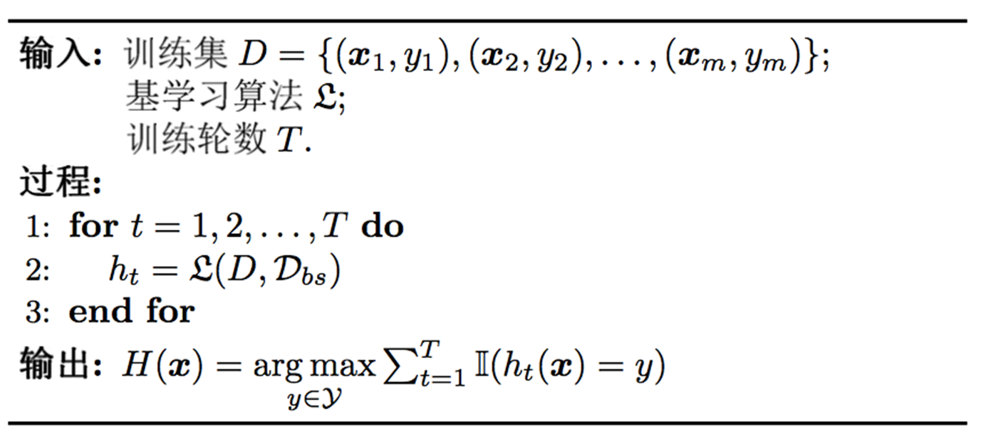
Adaboost
AdaBoost推导
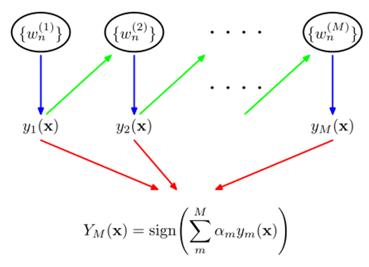
基学习器的线性组合
\[H(x)=\sum\limits_{t=1}^Ta_th_t(x)\]最小化指数损失函数
\[\mathcal{l}_{exp}(H\vert \mathcal{D})= \mathbb{E}_{x\sim\mathcal{D}}[e^{-f(x)H(x)}]\]其中 $\mathbb{E}_{x\sim\mathcal{D}}$ 表示对数据集 $D$ 以 $\mathcal{D}$ 的概率分布加权后的期望; $f(x)\in{1,-1},h(x)\in{1,-1}$
若 $H(x)$ 能令指数损失函数最小化,则上式对 $H(x)$ 的偏导值为0,即
\[\frac{\partial \mathcal{l}_{exp}(H(x)\vert\mathcal{D})}{\partial H(x)}=-e^{-H(x)}P(f(x)=1\vert x) +e^{H(x)}P(f(x)=-1\vert x)=0\\ \Longrightarrow\\ H(x)=\frac{1}{2}\ln\frac{P(f(x)=1\vert x)}{P(f(x)=-1\vert x)}\\ sign(H(x))=sign(\frac{1}{2}\ln\frac{P(f(x)=1\vert x)}{P(f(x)=-1\vert x)})\\ =\left\{ \begin{aligned} & 1,\quad P(f(x)=1\vert x)>P(f(x)=-1\vert x)\\ & 1,\quad P(f(x)=1\vert x)<P(f(x)=-1\vert x) \end{aligned} \right.\\ \mathop{\arg\max}\limits_{y\in\{-1,1\}}P(f(x)=y\vert x)\]$sign(H(x))$ 达到了贝叶斯最优错误率,说明指数损失函数是分类任务原来0/1损失函数的一致的替代函数
当基分类器 $h_t$ 基于分布 $D_t$ 产生后,该基分类器的权重 $\alpha_t$ 应该使得 $\alpha_th_t$ 最小化指数损失函数
\[\begin{aligned} \mathcal{l}_{exp}(\alpha_th_t\vert D_t) &= \mathbb{E}_{x\sim\mathcal{D}_t}[e^{-f(x)\alpha_th_t(x)}]\\ & =\mathbb{E}_{x\sim\mathcal{D}_t}[e^{-\alpha_t}\Pi(f(x)=h_t(x))+e^{\alpha_t}\Pi(f(x)\ne h_t(x))]\\ & =e^{-\alpha_t}P_{x\sim \mathcal{D}_t}(f(x)=h_t(x))+e^{\alpha_t}P_{x\sim \mathcal{D}_t}(f(x)\ne h_t(x))\\ & =e^{-\alpha_t}(1-\epsilon_t)+e^{\alpha_t}\epsilon_t\\ \end{aligned}\\ \epsilon_t=P_{x\sim \mathcal{D}_t}(f(x)\ne h_t(x))\]推导权重分布参数 $\alpha_t$ :令指数损失函数导数为零,即
\[\frac{\partial\mathcal{l}_{exp}(\alpha_th_t\vert \mathcal{D}_t)}{\partial\alpha_t}=-e^{-\alpha_t}(1-\epsilon_t)+e^{\alpha_t}\epsilon_t\\ \alpha_t=\frac{1}{2}\ln(\frac{1-\epsilon_t}{\epsilon_t})\]对获得 $H_{t-1}$ 之后的样本分布进行调整,使得下一轮基学习器 $h_t$ 能够纠正 $H_{t-1}$ 的一些错误
\[\mathcal{l}_{exp}(H_{t-1}+h_t\vert \mathcal{D}) =\mathbb{E}_{x\sim\mathcal{D}_t}[e^{-f(x)(H_{t-1}+h_t)}]\]泰勒展开近似为
\[\mathcal{l}_{exp}(H_{t-1}+h_t\vert \mathcal{D})\simeq \mathbb{E}_{x\sim\mathcal{D}_t}[e^{-f(x)H_{t-1}} (1-f(x)h_t(x)+\frac{f^2(x)h_t^2(x)}{2})]\]于是,理想的基学习器:
\[\begin{aligned} h_t(x) &=\mathop{\arg\min}\limits_h\mathcal{l}_{exp}(H_{t-1}+h_t\vert \mathcal{D})\\ &=\mathop{\arg\min}\limits_h\mathbb{E}_{x\sim\mathcal{D}}[e^{-f(x)H_{t-1}}(1-f(x)h_t(x)+\frac{1}{2})]\\ &=\mathop{\arg\max}\limits_h\mathbb{E}_{x\sim\mathcal{D}}[e^{-f(x)H_{t-1}}f(x)h(x)]\\ &=\mathop{\arg\max}\limits_h\mathbb{E}_{x\sim\mathcal{D}}[\frac{e^{-f(x)H_{t-1}}}{\mathbb{E}_{x\sim\mathcal{D}}[e^{-f(x)H_{t-1}(x)}]}f(x)h(x)] \end{aligned}\]注意到 $\mathbb{E}{x\sim\mathcal{D}_t}[e^{-f(x)H{t-1}(x)}]$ 是一个常数
令 $\mathcal{D}_t$ 表示一个分布:
\[\mathcal{D_t}(x)=\frac{\mathcal{D}(x)e^{-f(x)H_{t-1}}}{\mathbb{E}_{x\sim\mathcal{D}_t}[e^{-f(x)H_{t-1}(x)}]}\]根据数学期望的定义,这等价于令:
\[\begin{aligned} h_t(x) &=\mathop{\arg\max}\limits_h\mathbb{E}_{x\sim\mathcal{D}}[\frac{e^{-f(x)H_{t-1}}}{\mathbb{E}_{x\sim\mathcal{D}}[e^{-f(x)H_{t-1}(x)}]}f(x)h(x)]\\ &=\mathop{\arg\max}\limits_h\mathbb{E}_{x\sim\mathcal{D}_t}[f(x)h(x)] \end{aligned}\]由 $f(x),h(x)\in{-1,1}$ 有:
\[f(x)h(x)=1-2\Pi(f(x)\ne h(x))\]则理想的基学习器
\[h_t(x)=\mathop{\arg\min}\limits_h\mathbb{x\sim\mathcal{D}_t}[\Pi(f(x)\ne h(x))]\]最终的样本分布更新公式
\[\begin{aligned} \mathcal{D}_{t+1}(x) &=\frac{\mathcal{D}(x)e^{-f(x)H_{t}}}{\mathbb{E}_{x\sim\mathcal{D}_t}[e^{-f(x)H_{t}(x)}]}\\ &=\frac{\mathcal{D}(x)e^{-f(x)H_{t-1}}e^{-f(x)\alpha_th_t(x)}}{\mathbb{E}_{x\sim\mathcal{D}_t}[e^{-f(x)H_{t}(x)}]}\\ &=\mathcal{D}_t(x)\cdot e^{-f(x)\alpha_t h_t(x)} \frac{\mathbb{E}_{x\sim\mathcal{D}_t}[e^{-f(x)H_{t-1}(x)}]}{\mathbb{E}_{x\sim\mathcal{D}_t}[e^{-f(x)H_{t}(x)}]} \end{aligned}\]省流:Adaboost使用指数损失函数期望最小化作为优化目标,将这个损失期望拆分成前优化器损失+当前优化器损失,构造和前优化器相关的采样分布,优化目标变成当前采样分布下当前优化器损失的最小化
AdaBoost注意事项
数据分布的学习
- 重赋权法
- 重采样法
重启动,避免训练过程过早停止
从偏差-方差的角度:降低偏差,可对泛化性能相当弱的学习器构造出很强的集成
Bagging 与随机森林
- 个体学习器不存在强依赖关系
- 并行化生成
- 自助采样法
算法特点
- 时间复杂度低
- 假定基学习器的计算复杂度为 $O(m)$ ,采样与投票/平均过程的复杂度为 $O(s)$ ,则bagging的复杂度大致为 $T(O(m)+O(s))$
- 采样和投票的时间几乎可以忽略
- 可使用包外估计
包外估计
$H^{oob}(x)$ 表示对样本 $x$ 的包外预测,即仅考虑那些未使用 $x$ 训练的基学习器在 $x$ 上的预测
\[H^{oob}(x)=\mathop{\arg\max}\limits_{y\in\mathcal{Y}}\sum\limits_{t=1}^T\Pi(h_t(x)=y)\cdot(x\notin D_t)\]Bagging泛化误差的包外估计为:
\[\epsilon^{oob}=\frac{1}{\vert D\vert}\sum\limits_{(x,y)\in D}\Pi(H^{oob}(x)\ne y)\]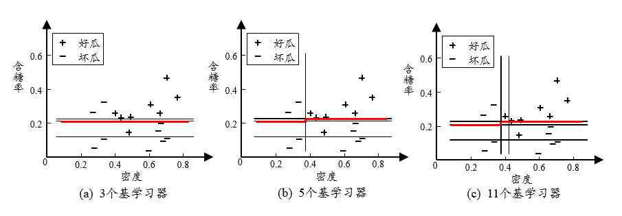
从偏差-方差的角度:降低方差,在不剪枝的决策树、神经网络等易受样本影响的学习器上效果更好
随机森林
随机森林(random forest,RF)是bagging的一个扩展变种 采样的随机性、属性选择的随机性:从属性中随机选择包含k个属性的子集,然后从k个属性中寻找一个最优划分的属性
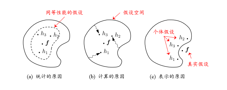
结合策略
学习器的组合可以从三个方面带来好处
平均法
简单平均法
\[H(x)=\frac{1}{T}\sum\limits_{i=1}^{T}h_i(x)\]加权平均法
\[H(x)=\frac{1}{T}\sum\limits_{i=1}^{T}w_ih_i(x)\]投票法
绝对多数投票法(majority voting)
\[H(x)= \left\{ \begin{aligned} & c_j & if\: \sum\limits_{i=1}^{T}h_i^j(x)>\frac{1}{2}\sum\limits_{k=1}^K\sum\limits_{i=1}^Th_i^k(x)\\ & rejection & otherwise \end{aligned} \right.\]相对多数投票法(plurality voting)
\[H(x)=c_{\mathop{\arg\max}\limits_{j}\sum\limits_{i=1}^Th_i^j(x)}\]加权投票法(weighted voting)
\[H(x)=c_{\mathop{\arg\max}\limits_{j}\sum\limits_{i=1}^Tw_ih_i^j(x)}\]学习法

多样性
误差-分歧分解
定义学习器 $h_i$ 的分歧(ambiguity):
\[A(h_i\vert x)=(h_i(x)-H(x))^2\]集成的分歧:
\[\begin{aligned} \bar{A}(h\vert x) &=\sum\limits_{i=1}^Tw_iA(h_i\vert x)\\ &=\sum\limits_{i=1}^Tw_i(h_i(x)-H(x))^2\\ \end{aligned}\]分歧项代表了个体学习器在样本x上的不一致性,即在一定程度上反映了个体学习器的多样性,个体学习器和集成的平方误差分别为
\[E(h_i\vert x)=(f(x)-h_i(x))^2\\ E(H\vert x)=(f(x)-H(x))^2\]令 $\bar{E}(h\vert x)=\sum\limits_{i=1}^Tw_iE(h_i\vert x)$ 表示个体学习器误差的加权平均
\[\begin{aligned} \bar{E}(h\vert x) &=\sum\limits_{i=1}^Tw_iE(h_i\vert x)-E(H\vert x)\\ &=\bar{E}(h\vert x)-E(H\vert x)\\ \end{aligned}\]令 $\bar{E}$ 表示个体学习器泛化误差的加权平均值, $\bar{A}$ 表示个体学习器的加权分歧值,有
\[E==\bar{E}-\bar{A}\]个体学习器的精确度越高、多样性越大,则集成效果越好,称为误差-分歧分解
多样性度量
多样性度量(diversity measure)用于度量集成中个体学习器的多样性
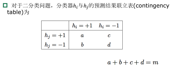
常见的多样性度量
- 不合度量(disagreement measure)
- 相关系数(correlation coefficient)
- Q-统计量(Q-Statistic)
- K-统计量(Kappa-Statistic)
多样性扰动
常见的增强个体学习器多样性的方法
- 数据样本扰动
- 基于采样法,Bagging中的自助采样法、Adaboost中的序列采样
- 对数据样本扰动敏感的基学习器(不稳定基学习器):决策树、神经网络
- 对数据样本扰动不敏感的基学习器(稳定学习器):线性学习器、SVM、朴素贝叶斯、k近邻
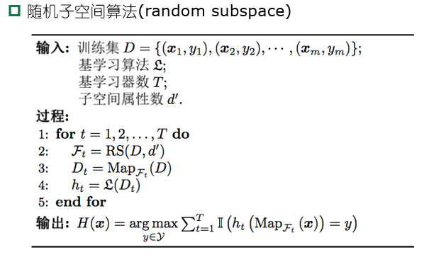
- 输入属性扰动
- 输出表示扰动
- 翻转法(flipping output)
- 输出调剂法(output smearing)
- ECOC法
- 算法参数扰动
- 负相关法
- 不同的多样性增强机制同时使用